Abstract

For digitally beamformed phased arrays, a common implementation method considered for the LO generation is to distribute a common reference frequency to a series of phase-locked loops distributed within the antenna array. With these distributed phase-locked loops, a method for assessing the combined phase noise performance is not well documented in current literature.

In a distributed system, common noise sources are correlated and distributed noise sources, if kept uncorrelated, are reduced when RF signals are combined. This is intuitive to assess for most components in the system. For a phase-locked loop there are noise transfer functions associated with every component in the loop, and their contribution is a function of the control loop and also any frequency translation. This adds complexity when attempting to assess a combined phase noise output. By building upon known phase-locked loop modeling methods, and an assessment of correlated vs. uncorrelated contributors, an approach to track distributed PLL contributions across frequency offsets is presented.

Introduction

In any radio system, careful design effort is placed on the implementation of the local oscillator (LO) generation for the receivers and exciters. With the proliferation of digital beamforming in phased array antenna systems, the design becomes additionally complicated with the distribution of LO signals and reference frequencies to a large number of distributed receivers and exciters.

A trade-off at the system architecture level is to distribute the LO frequencies needed or to distribute a lower frequency reference and to create the LO needed in close physical proximity to the point of use. A readily available and highly integrated option to create the LO locally is through a phase-locked loop. The next challenge is to assess a system-level phase noise from a variety of distributed components, as well as centralized components.

A system with distributed phase-locked loops can be considered as in Figure 1. A common reference frequency is distributed to many phase-locked loops each creating an output frequency. The LO outputs of Figure 1a are assumed to be the LO inputs to the mixers in Figure 1b.

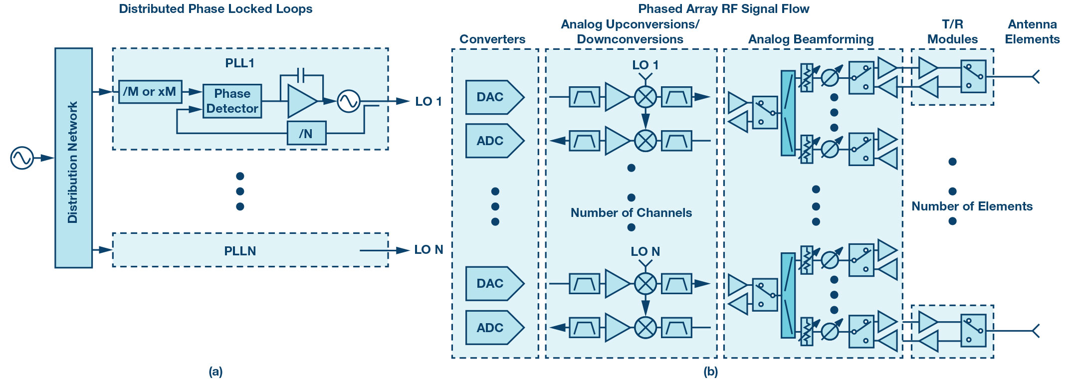
Figure 1. A system of distributed phase-locked loops. Each oscillator is phase-locked to a common reference oscillator. The LO signals, 1 to N, are applied to the LO ports of the mixers shown in the phased array.

A challenge for the system designer is tracking the noise contributions of the distributed system, understanding correlated vs. uncorrelated noise sources, and making an estimate of the overall system noise. In a phase-locked loop this challenge is compounded by noise transfer functions that are both a function of the frequency translation and loop bandwidth settings in the phase-locked loop.

Motivation: A Measured Example of Combined Phase-Locked Loops

An example measurement for combined phase-locked loops is shown in Figure 2. This data was taken by combining transmit output from multiple ADRV9009 transceivers. Cases for a single IC, two combined ICs, and four combined ICs are shown. In the case of this data set, there is a visible 10logN improvement as ICs are combined. In order to achieve the result a low noise crystal oscillator reference source was needed. The motivation to the model in the next section is to derive a method to calculate how this measurement would scale in a large array with many distributed transceivers and more generally to any architecture with distributed phase-locked loops.

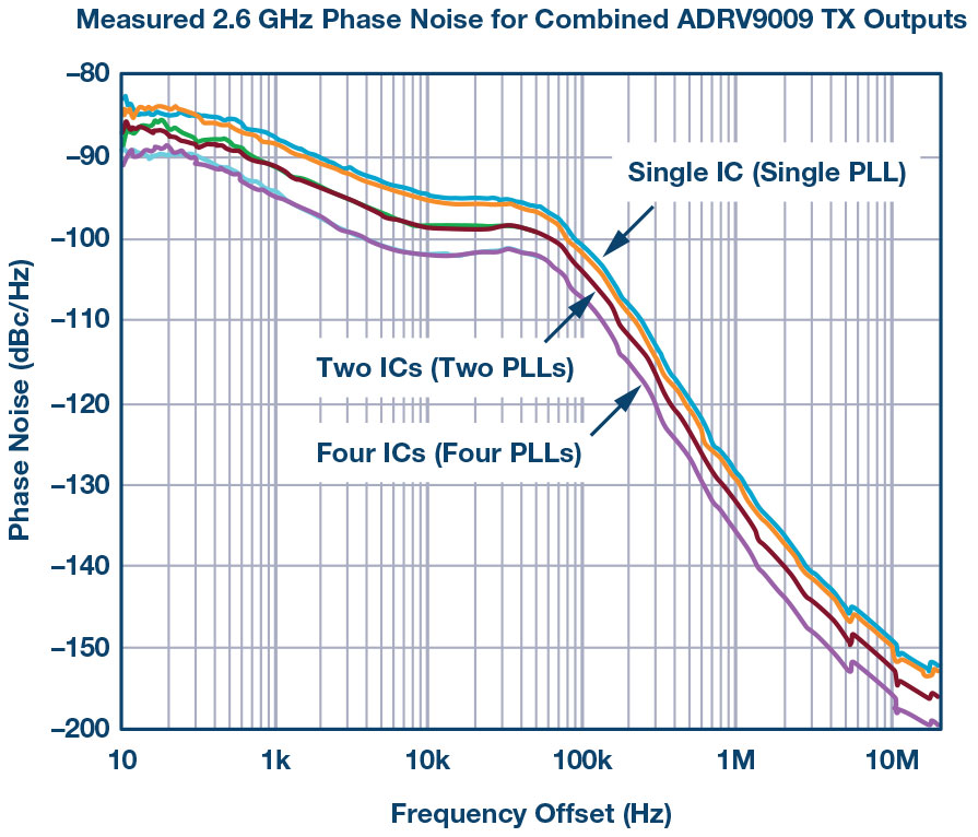
Figure 2. Phase noise measurement of combined two phase-locked loops.

Phase-Locked Loop Model

Noise modeling in phase-locked loops is well documented.1–5 An output phase noise plot is shown in Figure 3. In this type of plot, noise contributions for every component in the loop can be quickly assessed by the designer, and the accumulation of these contributors leads to the overall noise performance. The model parameters were set to be representative of the data shown in Figure 2, and the source oscillator used to create a phase noise estimate if a large quantity of ICs were to be combined.

To examine the effect with a distributed phase-locked loop, first the reference contribution and the contribution from the remaining PLL components are exported from the PLL model.

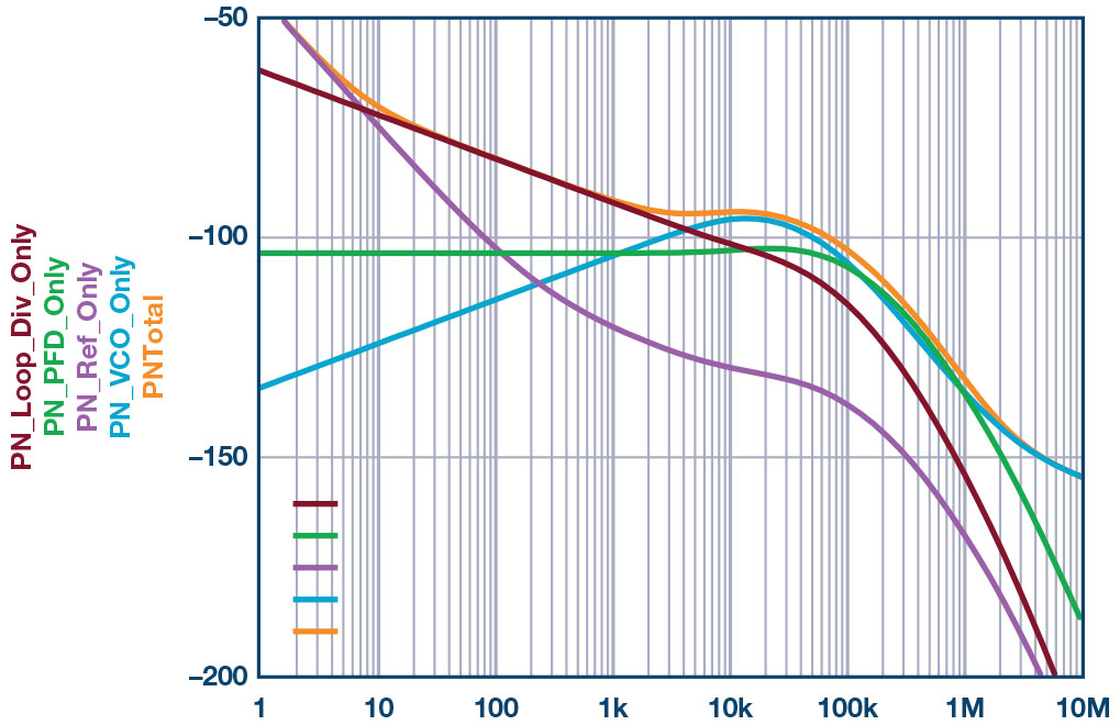
Figure 3. A typical phase-locked loop phase noise analysis showing the noise contributions of all the components. The total noise is the combination of all the contributors.

Extending Known PLL Models to Distributed PLL Models

Next, a process to calculate a combined phase noise for a system with many distributed phase-locked loops is described. This approach is based on being able to separate the noise contribution of the reference oscillator from the noise contributions of the VCO and loop components. Figure 4 illustrates a hypothetical distributed example of a single reference oscillator to many PLLs. This calculation assumes a noiseless distribution, which is not practical, but can be used to illustrate the principles. The noise contribution from the distributed PLL is assumed to be uncorrelated and reduced 10logN where N is the number of distributed PLLs. As channels are added, the noise is improved at larger offset frequencies and for large distribution systems the noise becomes almost completely dominated by the reference oscillator.

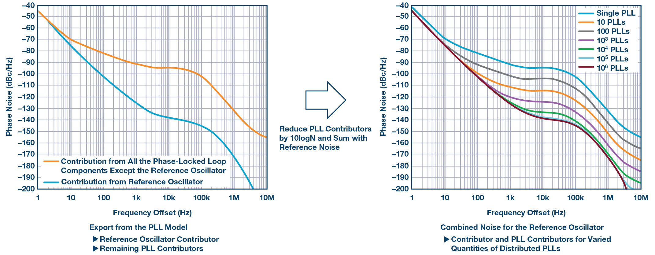
Figure 4. Beginning the distributed phase-locked loop phase noise modeling approach: the phase noise contributions of the reference oscillator and all the other components in the phase-locked loop except the reference oscillator are extracted from the PLL model. The combined phase noise as a function of the number of distributed phase-locked loops assumes that the reference noise is correlated and that the noise contributors distributed among many PLLs are uncorrelated.

The example illustrated in Figure 4 simplified assumptions on the reference oscillator distribution. In a true system analysis, it is expected that the system designer will also account for noise contributions in the reference oscillator distribution, which will degrade the overall results. However, a simplified analysis like this one is quite useful for gaining intuition on how architecture trade-offs may impact the overall system phase noise performance. Next we look at the impact of phase noise in the distribution system.

Accounting for Phase Noise in the Reference Distribution

Two examples of distribution options are evaluated next. The first case considered is shown in Figure 5. In this example, a wideband PLL is chosen that is common for the fast tuning of the VCO frequency. The distribution of the reference signal is implemented with clock PLL ICs that are also common to simplify timing constraints for digital data links such as JESD interfaces. Individual contributors are shown in the lower left. These contributors are at the frequencies of the device and are not scaled to the output frequency. The lower right phase noise plot shows the system-level phase noise for varying quantities of distributed PLLs.

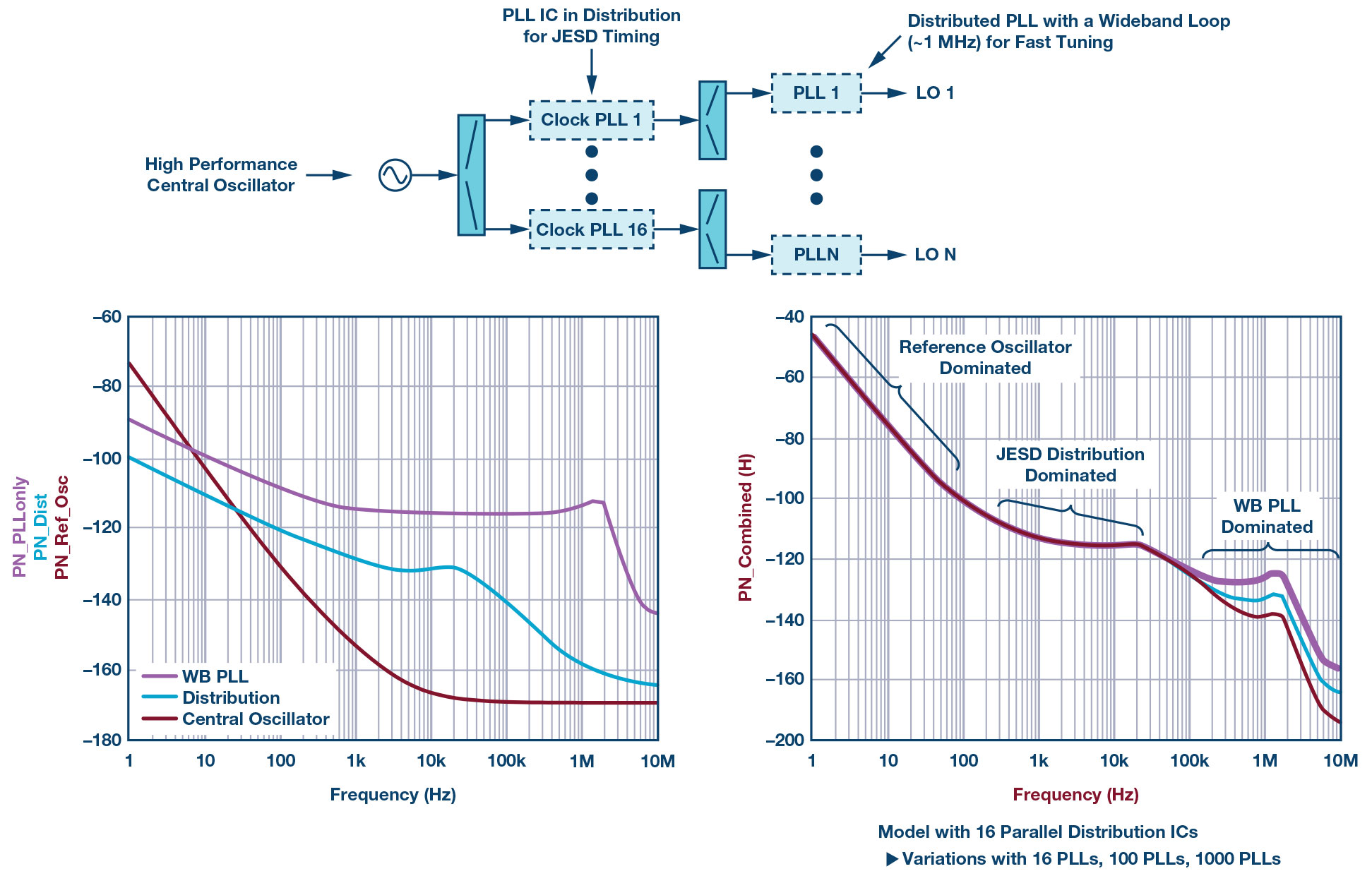
Figure 5. Distributed wideband PLL with a PLL IC in the distribution.

A few features about the model are worth noting. A single high performance crystal oscillator is assumed, nominally at 100 MHz, and the central oscillator individual contributor is reflected on what is available in reasonably high end crystal oscillators, although not necessarily the best and most expensive choice available. While the central oscillator output would be practical to fan out to a limited number of distribution PLLs, these would fan out again to some practical limit and repeat to serve the complete distribution in the system. For the distribution contribution in this example, 16 distribution components are assumed, then these are assumed to fan out again. The individual contribution of the distribution circuitry shown in the lower left is the noise of the PLL components without the reference oscillator contribution. The distribution in this example is assumed to be at the same frequency as source oscillator and noise contributors were chosen based on typical ICs available for this function.

The wideband PLL is assumed nominally at S-band frequencies, set to a 1 MHz loop bandwidth for fast tuning, which is about as wide a loop as is practical.

It is worth noting that these models were chosen to be typical of what might be practical and illustrate the cumulative effect in an array. Any detailed design may be able to improve a particular PLL noise curve, which is anticipated, and this analysis method is intended to aid the engineering decision of where to allocate design resources for the best overall result and is not intended to make an exact claim relative to available components.

The lower right plot in Figure 5 calculates the total combined phased noise for the LO distribution. PLL noise transfer functions of each individual contributor are applied, which both scales to the output frequency and includes the effect of the PLL loop bandwidth. The system quantities are also included and assumed to be uncorrelated and, thus, that contribution is reduced by 10logN. For the distribution quantity, 16 is assumed, as previously described, and the distribution contribution is reduced by 10log16. In practice this would degrade further as the distribution is repeated. However, the additional noise contribution is less significant. For a fanout distribution in a large array, the noise will be dominated by the first set of active devices. In the case of a fanout by groups of 16, such that each active device is the input to 16 more active devices, the additional distribution layer of 16 degrades only by ~0.25 dB if all are uncorrelated to each other. Continuing the distribution will have even less overall contribution. Therefore, to simplify the analysis, this effect is not included and the noise contribution of the distribution is calculated from the first 16 parallel distribution components.

The resulting curve illustrates several effects. Similar to a single PLL model, the close in noise is dominated by the reference frequency, the far out noise is dominated by the VCOs, and the far out noise improves as uncorrelated VCOs are added together. This is fairly intuitive. What is not intuitive, and the value of the model, is a large section of offset frequencies dominated by the choice made in the distribution. This result leads to considering a second example with a lower noise distribution and a narrower PLL loop bandwidth.

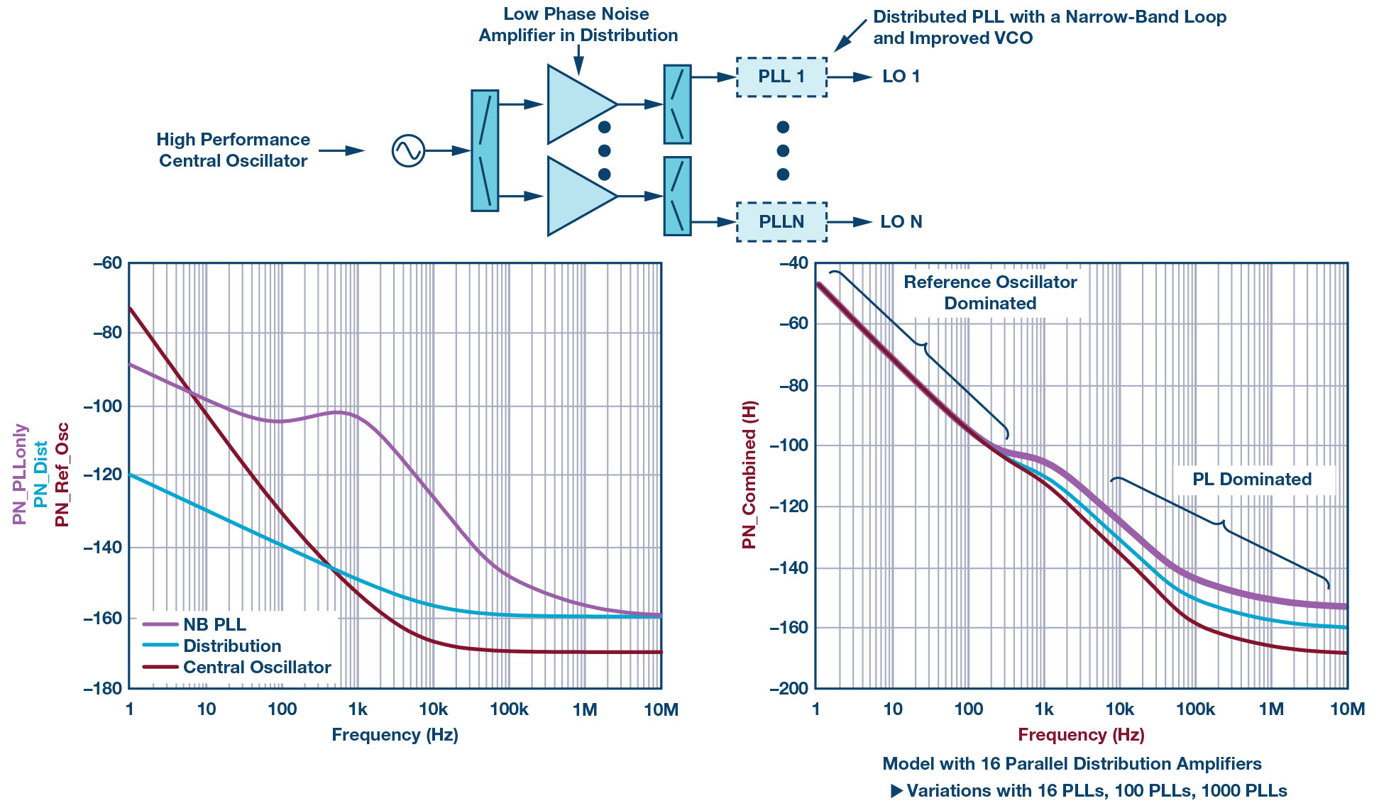
Figure 6. Distributed narrow-band PLL with amplifiers in the distribution.

Figure 6 illustrates a different approach. The same low noise crystal oscillator is used as a reference. This is distributed through RF amplifiers rather than retiming and resynchronizing through a PLL. The distributed PLL is chosen at a fixed frequency. This has two effects: at a single frequency with a narrow tuning range, the VCO can be intrinsically better, and the loop bandwidth can be made much narrower. The lower left plot shows the individual contributors. The central oscillator is the same as the previous example. Note the distribution amplifiers: they are not particularly high performance when considering low phase noise amplifiers, yet considerably better than using a PLL ICs such as the previous example. The distributed PLLs are improved at higher offset frequencies by both a better VCO and narrower loop bandwidth, but the mid frequencies of ~1 kHz are actually worse than the wideband PLL example. The lower right shows the combined result: the reference oscillator dominates the low frequencies, and above the loop bandwidth, the distributed PLL dominates performance and is improved with increasing the array size and quantities of distributed PLLs.

Figure 7 shows a comparison of the two examples. Note the wide range of differences in offset frequencies from ~2 kHz to 5 kHz.

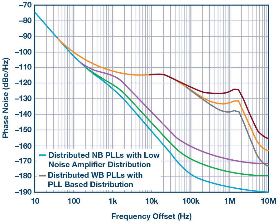
Figure 7. A comparison of Figure 5 and Figure 6 that illustrates the wide range of system-level performance dependent on the distribution and architecture chosen.