

Introduction
The importance of reliability can be best demonstrated using an anecdote I was told by a friend back in 2008; when working for a major IC firm from San Francisco, he had received a shipment of new and somewhat problematic desktop PCs.
Within months these PCs had started to crash, with the IT department being rolled in to fix the assumed operating system gremlins and / or viruses that were affecting these new computers – to no effect. After much investigation, and with many a stripped down PC, it was eventually revealed that the problem was caused by substandard bulk capacitors in the ac-dc power supply. These had deteriorated in use, and were causing the supply rails to be out of regulation, producing the random crashes.
The episode highlights that, while power supplies may not have the glamour, nor get the attention that processors and displays receive, they are just as vital to system operation. Here we look at reliability in power supplies, how it’s measured and how it can be improved.
Predicting the power supply’s expected life
First, a few definitions:
Reliability, R(t): The probability that a power supply will still be operational after a given time
Failure rate, λ: The proportion of units that fail in a given time, note, there is a high failure rate in the burn-in and wear-out phases of the cycle – see figure 1
MTTF, 1/λ: The mean time to failure.
MTBF (mean time between failures) is also commonly used in place of MTTF and is useful for equipment that will be repaired and then returned to service. MTTF is technically more correct mathematically, but the two terms are (except for a few situations) equivalent and MTBF is the more commonly used in the power industry.
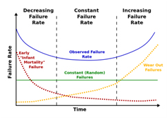
Figure 1: The bathtub curve, failure rate plotted against time with the three life-cycle phases: infant mortality, useful life and wear-out.
A supply’s reliability is a function of multiple factors: a solid, conservative design with adequate margins, quality components with suitable ratings, thermal considerations with necessary derating, and a consistent manufacturing process.
To calculate reliability – the probability of a component not failing after a given time – the following formula is used:
R(t) = e-λt
For example, the probability that a component with an intrinsic failure rate of 10-6 failures per hour wouldn’t fail after 100,000 hours is 90.5%, after 500,000 this decreases to 60.6%, and after 1 million hours of use this decreases to 36.7%.
Going through the mathematics can reveal interesting realities. First, the failures for a constant failure rate are characterized by an exponential factor, so only 37% of the units in a large group will last as long as the MTBF number; second, for a single supply, the probability that it will last as long as its MTBF rating is only 37%; and third, there is a 37% confidence level likelihood that it will last as long as its MTBF rating. Additionally, half the components in a group will have failed after just 0.69 of the MTBF.
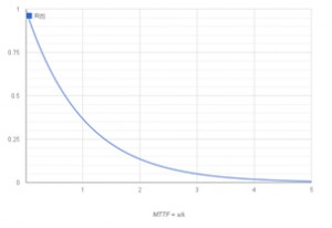
Figure 2: Curve showing the probability that a component is still operational over time.
It should also be noted that this formula and curve can be adapted to calculate the reliability of a system:
R(t) = e-λAt
Where λA is the sum total of all components failure rates (λA = λ1n1 + λ2n2 + … + λini)
Calculating the failure rate
Three methods can be used to calculate failure rates, prediction (during design), assessment (during manufacturing) and observation (during service life).
Prediction uses a standard database of component failure rates and expected life, typically MIL-HDBK-217 for military and commercial applications or Telcordia for telecom applications.
The MIL approach requires use of many parameters for the different components and includes voltage and power stresses, while Telcordia requires fewer component parameters and can also take into account lab-test results, burn-in data, and field-test data. Finally, the MIL approach yields MTBF data, while Telcordia produces FIT numbers, (failures per billion hours).
Using these databases and techniques means several, often incorrect, assumptions need to be made, such as the assumption that the design is perfect, the stresses are all known, everything is operated within its ratings, any single failure will cause complete failure, and the database is current and valid.
But, it is the least time consuming method and by applying it consistently across different designs, it can indicate the relative reliability of topologies and design approaches, rather than absolute reliability.
Conversely, assessment is the most accurate way of predicting failure rate, but requires greater time and resources. This method subjects a suitable number of final units to an accelerated life test at elevated temperature, with carefully controlled and increased stress factors.
One method, the HALT (highly accelerated life test) approach, tests a number of prototype units under as many conditions as possible, with cycling of temperature, input voltage, output load, and other impacting factors. HALT testing seeks to fatigue a component, PCB, subassembly, or finished product through either intense stressing for fewer cycles, or low level stressing for more cycles.
A second method, HASS (highly accelerated stress screen) testing is an accelerated reliability screening technique used to reveal latent flaws not detected by environmental stress screening, burn-in, or other test methods. HASS testing uses stresses beyond initial specifications, but still within the capability of the design as determined by HALT.
The stresses in HASS are more rigorous than those delivered by traditional approaches, so HASS testing substantially accelerates early discovery of manufacturing-process issues. Reliability engineers can then correct the variations that would otherwise lead to field failures and greatly reduce shipment of marginal product.
Observation in the field is also possible, but this is more difficult as it is impossible to control all of the conditions a supply has been subjected to and therefore more difficult to undertake reliable causation analysis.
Stresses that affect power supply reliability
Power supply life is affected by three kinds of stress: thermal, mechanical, and electrical. A quality design anticipates each of these and takes necessary steps to minimize both their occurrence and their impact.
Thermal stress takes two forms: static and dynamic. Static thermal stress, where supplies are operated at elevated temperatures, degrades components and their basic materials. Bulk capacitors may begin to dry out, or their seals may be stressed, and even resistor coatings may begin to deteriorate and break down. Interconnection and mating areas can expand and mismatch.
Dynamic stress is associated with the heating and cooling cycles and the resulting expansion / contraction, which leads to micro-cracks.
Mechanical stress severity depends on how and where the supply will be installed and used. This stress can cause both intermittent and hard failures, as cracks develop and circuit connections start to open and, in some cases, reconnect.
Electrical stress is any voltage, current, etc. that is applied to a device. Over- stress occurs when a component is operated beyond its rated value, either through poor selection or one-time events. For example, a capacitor may be rated to 100 VDC, but sees a 150 VDC spike in operation.
Improving power supply reliability through design
Obviously, the paper design and topology should be robust and cautious. This should take into account the effects of load and line transients, as well as noise. The designer should also carefully determine the required minimum/maximum values of component parameters to ensure reliable operation (a “typical” value is nearly meaningless), as well as those for critical second- and third-tier parameters; including less-publicized factors in the magnetic components, such as temperature coefficient of some values.
We’ve discussed the need to manage operational temperatures and a thermal analysis of the design and its physical implementation is therefore critical.
SPICE (simulation program with integrated circuit emphasis) or similar modeling of the design is essential, using realistic, not simplified, models of the components and PC boards and tracks, to verify both static and dynamic performance. And, the choice of components must be done with conservative bias, with extra margin in both initial and long-term values for many of their specification values. Furthermore, the layout must accommodate the fact that most supplies are dealing with significant current flows, on the order of 10, 20 or more amps.
After design, the next critical step is selection of specific components. As it’s nearly impossible to distinguish a poorly made or counterfeit unit, vendor credibility is key. Furthermore, components must be compatible with the manufacturing process; with mounting tabs, sufficiently large connection points and heavy wire leads, or screw terminals where appropriate.
And, on the subject of design for manufacturability, even the basic soldering process used in supply construction is an area for consideration. While the common reflow-soldering temperature profiles are well established, the regulatory mandate for lead-free (Pb-free) components and solder also means that a different reflow soldering profile is needed and all components used must also be qualified to perform to specification after this higher reflow temperature and soak time.
Improving power supply reliability through over specification
In addition to a cautious electrical design, the power supply vendor can do many things to increase overall reliability.
Using components that are inherently more reliable – by their physics, their design, their materials, or their manufacturing and test process – can significantly reduce the overall risk but does add to the overall cost. In power supplies the most common failure point is the capacitor, and, therefore, using longer-life capacitors will have the greatest effect.
A second way is to introduce redundancy. As we can see in figure 3, the probabilities of more than one unit failing are quite low. For example, if the reliability of any single unit is 0.99, then the probability of both units failing is 0.9999 in an N=1 design.
As we have already stated, just 37% of supplies will be operational after the MTTF. However, by adding just one additional supply, 60% of systems will have at least one operating supply after the same time period has elapsed.
Taking this to extreme, we can calculate that if we incorporate five power supplies into the design, more than 50% of systems will be still have a functioning supply after twice the MTTF has elapsed.
The N+1 method brings higher up-front cost, but does allow for a hot-swap capability to replace the failed supply.
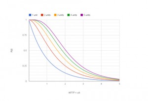
Figure 3: The effect of redundancy on the MTTF.
Additionaly, using components at levels well below their rated specifications is a relatively simple method of enhancing reliability.
If we look at temperature, a component rated for reliable operation at 85⁰C will have a significantly improved lifespan if used at 55⁰C – typically, a component’s life doubles for every 10⁰C decrease in temperature.
Minimizing temperature rise and temperature cycles is the most direct way to increase reliability, and this temperature-versus-life relationship is based on an adaptation of the Arrhenius equation:
AR = e((Ea/k).(1/T1-1/T2))
Ea = activation energy for the processes that lead to failure – typically 0.8eV to 1.0eV
k = Boltzman’s constant 8.617×10⁻⁵ ev k-1
T is temperature (oK), typically at ambient room temperature (298.15oK, 25oC)
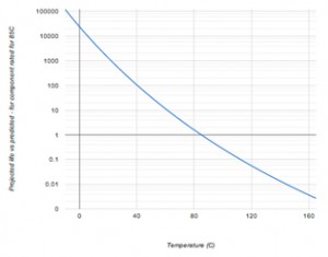
Fig 4: Effect of temperature on a component’s projected life. Plot is based on a component rated for 85oC and an activation energy (Ea) of 1.0
But, because it is dependent on how the customer mounts the supply, its enclosure, additional components in the enclosure, its ambient conditions, the use or non-use of active cooling such as fans, and other factors, this will often be beyond the OEM’s direct control.
Next on the list is burn-in testing. If we look back to figure 1, failure is significantly more likely during the early stages of a components life than it is during its useful life. Burn-in testing weeds out units that would have failed early in the field and therefore would have brought down the overall reliability rating.
Summary
Reliable supply design is not a guessing game. A reliable supply requires suitable design and analysis, components, manufacture process, test, and installation.
No single step will ensure a reliable supply, although there are many ways to decrease the supply’s reliability.
When a vendor analyzes the supply’s expected reliability, it is important to be consistent in databases, models, environmental conditions, and manufacturing in order to yield meaningful results, which can be compared across different power supplies and implementations.
At CUI we follow best practices to ensure our power supplies are among the industry’s most reliable. For further information on our power supplies and how they can be used to increase your system’s reliability visit www.cui.com.


